Putting DLI Data to Use: A Computing Exercise

Putting DLI Data to Use A Computing Exercise

The following exercise provides a hands-on computing experience that introduces some basic approaches to quantitative analysis. Included in a workshop that was first presented at the 1996 Learned Socieities Congress and sponsored by the Humanities and Social Sciences Federation of Canada, the computing tasks below use a data file consisting of a subset of variables and cases drawn from the national Survey of Literacy Skills Used in Daily Activities, 1989. Initially, this customized data file and the instructions accompanying the exercise were prepared for use with the NSDStat statistical system. Subsequently, these products were modified for use with the SPSS statistical package. To complete this exercise, you require the following:

  • a copy of the SPSS port file for the Literacy data,
  • a copy of the data documentation accompanying this file, and
  • access to the SPSS statistical package.

Becoming Familiar with the Data

Begin this exercise by familiarizing yourself with some of the variables in this customized data file. Using the accompanying data documentation, answer the following questions.

1. Below are some descriptions of variables appearing in the following statistical analyses. Identify the SPSS variable name for each item and then record the name in the table below. SPSS variables are specified under the ACRONYM field in the data documentation.

Which variable identifies province of residence?

Description SPSS Variable Name
Which variable captures the age of the respondents? .
Which variable captures how often the respondents went to a public library? .
Which variable contains the IRT Reading Ability score? .
Which variable contains the four categorized reading levels? .

2. Use the data documentation to determine whether the following variables are categorical or analytic. The distinction between categorical and analytic measurement appears in Exploring Data Liberation. Knowing the measurement of a variable is important when considering the choice of a statistical procedure for an analysis. Check the column in the table below that matches each variable’s level of measurement.

Variable Name Measurement Level
Categorical Analytic
PROV . .
AGECLPSD . .
Q11C . .
Q22A . .
SEX . .
Q41 . .
IRT Reading Ability . .
Reading Level . .

Loading the Literacy Data File in SPSS

The customized file for this exercise has been saved as both an SPSS portable and system file. The system file, which was produced by processing the raw data in a previous SPSS/Windows session, contains just the data for the subset of cases and variables described in the accompanying data documentation. The system file is not readable by the eye but does include the data and all of the information declared for each variable, such as labels and missing values. The SPSS portable file is a text file version of this system file. However, the contents have been encoded to preserve the data and variable information in a format that is not machine dependent.

You must begin by retrieving a copy of either the portable or system file. Both are available at: ftp://datalib.library.ualberta.ca/pub. The SPSS system file is named dlilit89.sav while the portable version is named dlilit89.por. If you are using SPSS/Windows, the system file is the appropriate choice although the portable file also works. If you are using SPSS on any system other than Windows, retrieve only the portable file. Below is an example of retrieving a copy of the system file using ftp:

ftp datalib.library.ualberta.ca
anonymous
e-mail address
cd pub
binary
hash
get dlilit89.sav
quit

To load either the portable or system file in SPSS for Windows, begin the SPSS program and select the File option from the menu at the top of the SPSS window.
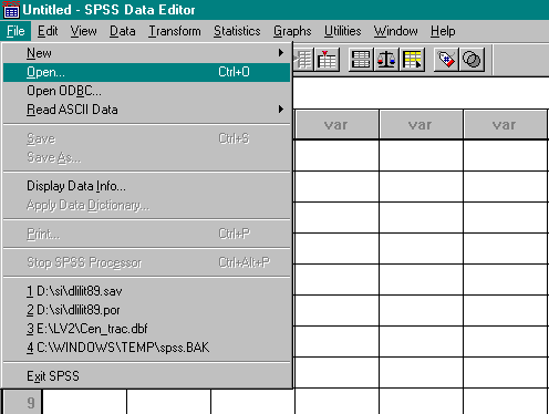
 

safile.gif

Next, select the Open option and specify the file type and location of the file on your machine.
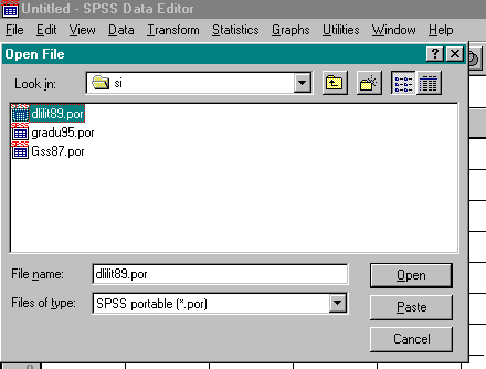
saopen.gif

In the example shown, the file dlilit89.por in the directory si has been identified and declared as an SPSS portable file. Clicking on OPEN will load the data from this file into the current Data Editor (as shown in the following figure.)
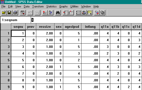
salit89

You are now ready to complete the data analysis described below.

Descriptive Statistics: Working with Categorical Variables

Analysis Objective. When pursuing background about a policy issue, one question often asked is, “How big will be the impact?” Similarly, when investigating a social problem, the question typically becomes, “How many people face this problem?” One approach to answering either of these questions is to compute population estimates of the focal group. An estimate will provide some sense about the scale of the social problem or the impact of a particular social policy.

Analysis Issue. One concern in the late 80’s was the estimate of functional illiterates in Canada. Southam Press had conducted research in 1987 that suggested one in four adults in Canada were functionally illiterate. Statistics Canada conducted their own survey in 1989 to address this issue.

Using the summary variable for reading ability level (RDLEVELA) in the file loaded above, obtain population estimates for this variable. Initially, the frequencies for variables in this file are based on the sample size, that is, the number of respondents in this survey. Statistics Canada, however, has provided a variable that weights cases (1) to adjust for the sampling methodology employed in gathering the data and (2) to provide population estimates. Because not every case in the study had the same probability of being selected for this survey, a weight variable was added to correct for unequal probabilities. In addition, these corrections also rescale the frequencies to an estimate of the population from which the sample was drawn.

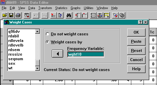
Exercise. To use the Statistics Canada weight variable in an analysis, SPSS must first be instructed to perform weighting and assigned the variable containing the weight values. In this instance, the name of the Statistics Canada weight variable is WGHT10. The script for making this assignment in SPSS is given below.

Determining a Population Estimate

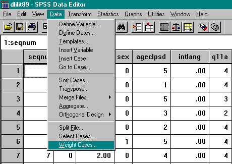
From the menu bar, select Data and then Weight Cases.
sbdawt.gif

Click on the button to select “Weight cases by” and insert the variable WGHT10.
sbdawt2

Click OK

You are now ready to obtain the frequencies for the reading level variable.

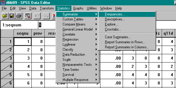
Select from the menu bar Statistics-Summarize-Frequencies and request the frequency distribution for RDLEVELA.
sbst1

Complete the following information using the output on your monitor for the frequency distribution of RDLEVELA.

Total Weighted N =
Number of Missing Cases =
RDLEVELA Number or Frequency Valid Percent
Level 1 . .
Level 2 . .
Level 3 . .
Level 4 . .

Population Estimates Using the Approximate Variance Table

To work with population estimates from this study, Statistics Canada provides guidelines in its data documentation that should be followed. An example for reporting a population estimate for Level 1 reading ability using their guidelines is provided next. To complete this exercise, you will need to use both the Approximate Variance Table for Canada and the Sampling Variability Guidelines included in the data documentation accompanying this study.

Step Instruction Answer
Step 1 Record the weighted frequency for Level 1: .
Step 2 Round the figure in Step 1 nearest 1,000: .
Step 3 Using the Approximate Variance Table, look down the far left column the number closest to the figure in Step 2 (the table lists values in ‘000). Follow the string of asterisks to the right until you encounter a number. Record the value from this table: .
Step 4 Using the Sampling Variability Guidelines, compare the figure recorded in Step 3 with the table in the guidelines. How should the population estimate for Level 1 be reported according to the guidelines? .

Confidence Intervals Using the Approximate Variance Table

In the above exercise, you estimated a count in thousands. While the computer generated a precise number, the answer was rounded to the nearest thousand. This is done to avoid a sense of greater precision than exists. An alternative to reporting an exact count is to report a confidence interval, usually a 95% interval. In working with a confidence interval, one reports a range within which one believes the population value to exist. Thus, one would report that 19 out of 20 times, one would expect the confidence interval to contain the population count. Public opinion poll results are often reported using this approach. For example, a poll might reveal that 45% of the public would vote for the Liberal Party if an election were held today, plus or minus 4%, 19 out of 20 times. In other words, one would expect the Liberals to receive between 41% and 49% of the vote if the election were held on the day of the poll, where 41% is the lower confidence interval (45%-4%) and 49% is the upper confidence interval (45%+4%).

Using the above results for reading ability level, calculate a confidence interval for one of the percentages. This will entail a bit of simple arithmetic.

Step Instruction Answer
Step 1 Record the percentage of the population with a Level 3 reading ability level: .
Step 2 Convert the percentage into a proportion by dividing by 100, i.e., move the decimal point two places to the left and record the value: .
Step 3 Enter the weighted frequency for Level 3: .
Step 4 Round the figure in Step 3 nearest 1,000: .
Step 5 Using the Approximate Variance Table, look down the far left column for the number closest to the figure in Step 4 (remember the table lists values in ‘000). Follow the string of asterisks to the right until you encounter a number. Record the value from this table: .
Step 6 Convert the percentage in Step 5 to a proportion by dividing by 100, i.e., move the decimal point two places to the left and record the value: .
Step 7 A 95% confidence interval (CI95) brackets a parameter estimate and thus, consists of two values: an interval minimum and maximum. To calculate these values, complete the following equations:

CI95 minimum = .222 – ( 2 * .222 * .033), where .222 comes from Step 2, the 2 in parentheses is the approximate value for the 95% level and .033 is the coefficient of variation from Step 6.

CI95 maximum = .222 + ( 2 * .222 * .033)

.

In interpreting the results, one would conclude that the percentage of adult Canadians with a reading ability at level three lies between 20.7% (the lower confidence interval) and 23.7% (the upper confidence interval).

Using a Subset of Cases and Calculating a Confidence Interval

The next exercise entails examining the distribution of the reading ability levels of just those respondents who have completed some secondary education. To approach an analysis in this way, one is looking at a special subpopulation and examining key dependent variables of this group. For example, what is the reading ability level of those who have some secondary education but who did not receive a secondary degree? This is what we will explore.

Turn to the data documentation and find the variable containing the respondent’s highest level of education. Next, identify the code used to classify those who “completed some secondary education.” Record your answers here.

Variable Name of Respondent’s Highest Level of Education Code for the Category: Completed Some Secondary Education:
. .

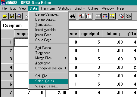
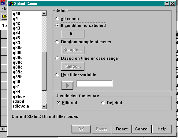
From the menu bar, select Data and Select cases.
sbdasl

Select the button displayed as: If condition is satisfied
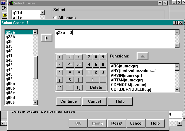
Press the IF button, which was activated by the previous step.
sbdasl2

Select Q22A and complete the equation as follows: Q22A = 3
sbdasl3

Click Continue and and then OK.

Notice that Filter On is reported below the horizontal scroll bar, which indicates a case selection is in effect.

Run the frequencies for RDLEVELA and complete the following table below.

Total Weighted N =
Number of Missing Cases =
RDLEVELA Number or Frequency Valid Percent
Level 1 . .
Level 2 . .
Level 3 . .
Level 4 . .

Using these results, calculate a confidence interval for the proportion with a Level 2 reading ability. Notice that using a subpopulation entails interpreting the Approximate Variance Table differently than the two previous exercises (see Step 5 below).

Step Instruction Answer
Step 1 Record the percentage of those with a Level 2 reading ability level: .
Step 2 Convert the percentage into a proportion by dividing by 100, i.e., move the decimal point two places to the left and record the value: .
Step 3 Enter the weighted frequency for Level 2: .
Step 4 Round the figure in Step 3 nearest 1,000: .
Step 5 Using the Approximate Variance Table, look down the far left column for the number closest to the figure in Step 4 (remember the table lists values in ‘000). Next, move across the columns at the top of the Table until you find a percentage close to the value in Step 1. The figure that intersects this row and column is the coefficient of variation to be used. Record the Table value: .
Step 6 Convert the percentage in Step 5 to a proportion by dividing by 100, i.e., move the decimal point two places to the left and record the value: .
Step 7 Calculate upper and lower 95% CI:

CI95 min = a – ( 2 * a * b), where a = the proportion from Step 2 and b is the coefficient of variation from Step 6.

CI95 max = a + ( 2 * a * b), where a = the proportion from Step 2 and b is the coefficient of variation from Step 6.

.

Re-select All Cases and Change Weight Variables

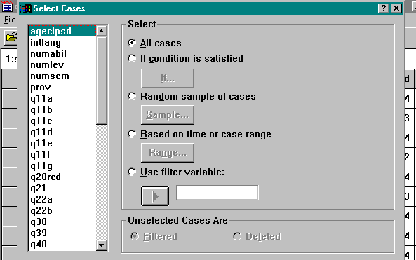
Next, turn off the filter that selected the subpopulation defined above so that subsequent analyses will use all of the cases. From the menu bar, select Data, Select Cases, then choose the button for All cases, and click OK.
scsel

The above weight variable not only corrected for the sampling methodology, but also produced population estimates. There are times when population estimates are not really required. Instead of wanting to know an estimate of the number of people in Canada with a certain attribute, the research focus is on the proportion or average of some property. Nevertheless, a weight variable is still required to adjust for the sampling methodology. Without this adjustment, the results cannot be generalized to the population. A second weight variable has been included with the Literacy work file that re-scales the weight variable back to the sample size, that is, to the size of the original sample rather than the estimated population size.

Now change the weight variable to the re-scaled weight variable, which is named, WT. From the menu bar, select Data, Weight Cases, replace WGHT10 with WT, and click OK.
Descriptive Statistics: Working with Analytic Variables

Putting DLI Data to Use

EXPLORING DATA LIBERATION
Putting DLI Data to Use

Workshop Objectives

The two primary goals of this workshop are (1) to present an example of working with data that uses one of the files available through the Data Liberation Initiative and (2) to provide a hands-on computing exercise that introduces some basic approaches to quantitative analysis. The study chosen for this example is the national Survey of Literacy Skills Used in Daily Activities conducted in 1989. The variety of variables in this study offer rich examples and its content features an important issue. In completing this example, three general strategies for performing quantitative analysis will be discussed.

In addition, this workshop is an initial small step in a much more ambitious plan to build a data culture in Canada. The concept of a data culture is one that foresees the widespread use of high-quality data by concerned citizens, policy analysts, educators and researchers in the general debate of societal issues. In this perspective, data are easily accessible to all interested parties and become an important element in shaping substantive positions on major issues confronting Canadians.

A Role for Quantitative Analysis

For the average person, quantitative analysis suffers from an association with higher mathematics or bean counting. One cannot escape the fact that quantitative analysis entails working with numbers. However, the level of mathematical background that is required varies greatly. As discussed below, numeric summaries are commonly being represented today in graphical displays. If a person works well with visual summaries, there is little reason not to use data. The bottom line – to borrow a term from th e bean counters – is that quantitative analysis tends to intimidate many people and, consequently, to lessen the use of data. This is unfortunate because the real utility of quantitative analysis is in displaying relationships in data that challenge conventional wisdom or that confirm ideas about social phenomena.

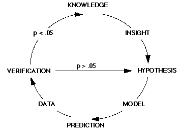
In its application, quantitative analysis is often introduced in the context of two separate paradigms: “doing science” or “making decisions”. Typical representations of these two paradigms are shown in Figures 1 and 2, respectively. Neither of these models explicitly identify a role for quantitative analysis. Instead, quantitative analysis appears as an implicit step following a “data step”. For example, the model of the traditional scientific method shown in Figure 1 implies some type of analysis between Data and Verification. Similarly, the decision-making model in Figure 2 contains an implicit analytic step in the link between Data and Information.
fig1sciFigure 1: Doing Science
From William Eddy, “Comments,” JASA (March 1979)

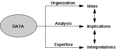
While the Data step does not appear as a dominant feature in either of the two paradigms, data nevertheless are an integral part in creating information or in verifying the correctness of the scientific model being tested. A useful way of viewing the process by which Data are transformed into information is shown in Figure 3. In this representation, Data are central to the model and are crucial to all other activities. Going in one direction, new ideas may be discovered if data are properly organized and displayed. In another direction, one or more implications may be drawn from an analysis of the Data. Third, interpretations may flow from the Data given specific expertise in combination with the implications of an analysis or the ideas from a display of the Data. Whether activities flow from the scientific method or a decision-making model, data and quantitative analysis play an important role. The next section discusses a framework for quantitative analysis.


fig2decFigure 2: Making Decisions

From William Bradley, et al., “Metadata Matters: standardizing metadata for improved management and delivery in national information systems,” (Social Environment Information Group, Health Canada), p. 17.

A Way of Viewing Quantitative Analysis

Performing quantitative analysis involves combining activities from three areas: statistics, data analysis, and social data. Each of these areas is discussed below.
fig3dataFigure 3: Data Focused Model
Adapted from William Eddy, op. cit.

Statistics

Statistics has a number of meanings and can refer to numeric facts, such as batting averages in professional baseball, or to a specialized branch of mathematics. To avoid confusion between its popular and technical usage, a clarification of its meaning is warranted.

The earliest definition of statistics in the Oxford English Dictionary refers to the activities of collecting, classifying, and discussing numeric facts about states or nations. This usage arose during the 18th Century coinciding with the emergence of the modern nation-state. The statistics mills of these nation-states amassed data for the decision-makers in the government of the day and for the administrators of bureaus and departments of government services and programs. Statistics Canada, in this regard, has been aptly named.

In recent use, statistics has become the science of generalization. Built upon theories of probability and inference, statistics permits broad generalizations from specific observations, whether related to human or natural phenomena. Instrumental in making generalizations are models and techniques that incorporate stochastic or error components. In this workshop, statistics refers to the methods and techniques for summarizing data and for estimating a variety of models of inference.

fig4comp

Figure 4: Components of Quantitative Analysis

Statistical Tools

Scores of statistical techniques and tools exist for analyzing data, which can prove to be overwhelming. This workshop will not present a comprehensive list of statistical techniques nor prescribe specific statistical tools. Rather, two points are offered. First, some statistical tools are more appropriately used with certain types of data. Secondly, many different statistical tools may be used to analyze the same set of variables with no one tool being more “right” or “wrong” than the other. There are clearly instances where it is inappropriate to apply certain statistical procedures, such as calculating the mean of marital status. But by the same token, there is not just one way of analyzing data. The tools and creativity applied to a particular analysis are part of the art of quantitative analysis.

We do offer, however, a brief summary of the more basic statistical techniques in Table 1. Again, the list is not comprehensive, but rather is illustrative of the match between statistical tools and data. In particular, two key properties of a set of variables help make this point. First, an analytic distinction is made between dependent and independent variables. This implies a causal relationship between variables, where the dependent variables represent the phenomenon being explained and the independent variables serve as the casual agents.

Not all quantitative analysis necessarily has to be conceived in terms of causality. For example, examining a single variable falls outside this context. Similarly, data reduction techniques do not require specifying dependent and independent variables, but instead are directed at identifying the shared measurement of a latent property, that is, an indirectly observed attribute. Factor analysis, latent class analysis and cluster analysis are methods commonly used for this purpose. Latent variables are further discussed below.

The second concept applied in Table 1 describes the observational representation of the data. Quantitative observations boil down to either counts or measurements. Variables in which observations are classified by a property, such as the sex or gender of a respondent, are analyzed by counting the number of observations within each category of the property, for example, the number of females, the number of males, and the number for whom sex was not identified. In our framework, variables consisting of a comprehensive set of mutually exclusive categories are identified as Categorical Variables. All variables in which the responses are a name or a proper noun fit this classification. A typical example of a categorical variable is sex, where the responses are ‘female’, ‘male’ or ‘unknown’. Similarly, marital status is a categorical variable with the possible responses being ‘single’, ‘married/common-law’, ‘separated/divorced’, ‘widowed’ or ‘unknown’.


Table 1: A Classification of Basic Statistical Tools

Independent Variables
Dependent Variables Categorical Analytic
Categorical Data Type: Frequencies or Count Data Type: Biserial Correlation
Methods: Tables, Loglinear Analysis Latent Class analysis Methods: Probit/Logit, Discriminant Analysis
Analytic Data Type: Means and Variances Data Type: Correlation Matrices
Methods: Analysis of Variance, Multivariate ANOVA, T-Test Methods: Regression analysis, Factor analysis

Variables that capture some level of measurement, on the other hand, are called Analytic in our classification. The level of measurement may range from a rough ranking or ordering of a property to a fairly precise amount or quantity of the property. For example, self-attributed health status might be measured on an ordinal scale that increases as general health improves. The values for this variable might be ‘Poor’, ‘Fair’, ‘Good’, or ‘Excellent’. While these responses appear to fit the above description of a Categorical Variable, the responses are actually adjectives describing various states of health that increase as overall health status improves. When a variable’s responses consist of adjectives that describe an increase or decrease in the state of a property, the variable is usually treated as a weak Analytic Variable, weak because the measurement is not based on a metric, that is, a standardized unit.

Variables that have been measured using a metric capture a precise amount or quantity of a property. Personal income, where dollars are the metric of measurement, is an example of this type of Analytic Variable. Furthermore, one can speak of 0 dollars as being the absence of income. Someone earning $20,000 makes twice as much as someone earning $10,000. Also, a dollar difference between 5 and 6 dollars is the same amount as the difference between 100 and 101 dollars, namely, one dollar. These three attributes, an absolute zero, ratio comparisons, and equal intervals, are all characteristics of strong Analytic Variables.

Social Data

Social data produced by governmental departments, academic research and the private sector about Canadian society can be summarized according to four basic data structures: unit record files, also known as microdata releases (e.g., the Public Use Microdata Files from the 1991 Census); aggregate files (e.g., the basic summary tables from the Census); time series records (e.g., CANSIM records); and geo-referenced or spatial files (e.g., the Census geography files).

Among the unit record files, a variety of data collection methods have been employed, including one-time cross-sectional surveys (e.g., the Family History Survey), repeated surveys (e.g., the General Social Surveys), and longitudinal surveys (e.g., the National Population Health Survey). These methods differ according to how time is controlled or manipulated. A one-time cross-sectional survey permits examining phenomena at a discrete point in time. Generalizations about change are difficult to infer from this data collection method. Repeated surveys, on the other hand, permit comparisons over time among cohorts. Individual change is difficult to infer, but aggregate change within a group can be observed. Finally, longitudinal surveys allow the examination of change at the level of the individual. While this method of data collection may appear to be the most ideal for explaining social phenomena, longitudinal surveys present some of the more complex data analysis problems.

A massive volume of data is collected by our national statistical information system in Canada. While concerns may exist about the scope and detail of the social issues captured by this system, volume of data is not a contentious point. A significant barrier, however, has been access to these data. One may have expected technology to have been the major hindrance to using these data, but a more basic factor has been simply getting copies of the data files. Several barriers have prevented open access to these data, including cost, concern about disclosure and confidentiality, poor data management practices, and issues of ownership. DLI is a program that specifically addresses access for post-secondary, non-commercial use of a sizable quantity of Statistics Canada data files. Nevertheless, identifying data collections that are appropriate to a specific research project remains a challenge.

Two general problems confront the secondary analysis of previously collected data. First, there is the challenge of matching units of analysis. This entails locating data observed using the same unit of analysis as your research interest. Since a large percentage of social research focuses on individuals as the unit of analysis, Statistics Canada’s microdata files are an attractive source to examine. If your research, however, is about individuals from a special or rare population, none of the major microdata files may have enough cases to permit an analysis, or the information needed to identify the group of interest may not be present in the file. For example, someone interested in studying aboriginal women who use computers in the workplace may not find enough cases in any of the microdata files, or the variables that would allow the identification of these cases may not be in the microdata file. Research requiring the identity of smaller communities of less than 250,000 is particularly challenging since one method frequently used to protect the confidentiality of individuals when constructing microdata files is to report locations only for largely populated areas, such as CMA’s, or large geographic units, such as provinces.

The second general challenge is to find data files that have captured the subject matter or content of interest. Here the focus in on finding variables that address the research question at hand. The researcher will want to ensure both that the complete mix of dependent and independent variables is within a microdata file and also that the phenomenon being studied was measured or observed as desired. The latter concern raises the issue of manifest and latent variables. Variables that are directly observed are manifest variables, while latent variables represent phenomena that, while not directly observed, are believed to underlie observed variables. A phenomenon such as worker alienation may not be measured directly by any one variable, but instead may be an underlying dimension in the measurement of several variables, including work satisfaction, salary level, relations with co-workers and management, personal goals, opportunities for advancement, etc. As mentioned above, some statistical techniques help abstract latent dimensions.

Data Analysis

Data analysis involves applying statistical computational techniques to social data. The advent of computer automation has revolutionized data processing and has introduced a number of new approaches in analyzing data. Access to computing power capable of processing public use microdata releases of the Census was once a serious concern for researchers. The current computing power of a notebook computer with an attached CD-ROM player can process these substantial files. However, it is not just the power of a briefcase-sized computer that makes possible the ability to process these large files. Equally important is the processing power of statistical software operating on today’s small computers. Major systems such as SAS and SPSS are available across the range of computing platforms and there are a number of smaller scaled packages that also carry a major processing punch, including NSDStat.

Data analysis includes data management operations necessary to organize a data file for statistical analysis. This entails identifying the observations in a file that are most appropriate for an analysis, which in some instances requires defining and extracting a subset of the observations from the original file. In other instances, the structure of the file may have to be aggregated to achieve the proper unit of analysis, for example, job-level observations in the Labour Market Activity Surveys may have to be summarized to create person-level records.

In addition to working with the case or observation structure of a file, data management tasks also involve strategies in manipulating or transforming variables. This includes creating new variables from existing variables or combining categories in an existing variable, for example, grouping age into five to ten year intervals. Together, case and variable manipulation play an important role in the completion of an analysis.

Quantitative Analysis Strategies: Description, Comparison, Modeling

The intersection of these three areas – statistics, social data, and data analysis – focuses our attention on quantitative analysis strategies. Such strategies consist of the variety of ways in which data files, statistical tools, and data management techniques are combined. While the only limitation to strategies appears to be ones creativity, three general approaches are most commonly employed: description, comparison, and modeling. Examples of these three approaches are provided in the accompanying computing exercise and each is discussed briefly below.

Description: summary of a sample or data collection

There are times when the primary purpose of an analysis is simply to describe the characteristics of a certain subpopulation or special group. Three types of numeric summaries are especially useful in these instances. First, accurate population estimates may be desired. While the data will be descriptive of the time period for which they were gathered, this information may be useful in describing or identifying the approximate size of a group or severity of a problem. Statistics Canada typically provides a variable (commonly referred to as a weight variable) that will produce population estimates from their sample. For example, the sample size for the number of women in the 1989 Survey of Literacy Skills Used in Daily Activities is 4,600. The population estimate applying the Statistics Canada weight variable is 7,284,422 women.

Because a population estimate is calculated from a sample, confidence intervals may be reported to provide a sense of the range of values within which the ‘true’ population value is likely to fall. Statistics Canada documentation often includes sampling variability tables that permit the calculation of a population estimate’s confidence interval. In many ways, a confidence interval is more meaningful to discuss than an actual population estimate because of natural fluctuations within social phenomena.

The useful second numeric summary is based on the relative size of categories within a Categorical Variable. Percentages are typically used for this purpose. For example, instead of reporting that 12,301,788 Canadians were married in 1991, this fact is reported as 45.6 percent of Canadians. This figure adjusts the frequencies to a 100 point scale, which easily permits comparisons of the relative size of each category within a variable.

The third numeric summary often reported is a “typical value” (also known as a measure of central tendency) of an Analytic Variable, i.e., variables with a continuous distribution. The most common “typical values” are the mean and median, although, the most frequently occurring value (or mode) might also be reported. In summarizing a continuous distribution it is also important to know the spread of a distribution, i.e., how widely the values are dispersed along a variable’s continuous scale. The spread of a distribution may be reported as the range, i.e., the distance between the minimum and maximum values, or as the standard deviation of the mean.

Comparison: looking at difference in means and percentages

A second strategy involves comparing the summary figures, i.e., percentages or “typical values”, of important dependent variables across groups. Instead of describing a particular population or group, phenomena are examined by contrasting differences or similarities among groups.

The comparison approach is commonly used in controlled experiments. One group, designated the experimental group, is subjected to a change, while a control group receives no treatment. The outcome, which is measured in a key dependent variable, is then compared between the control and experimental groups to see if the treatment made a difference.

Since survey research rarely involves the use of experimental controls, statistical control of variables is used during an analysis of the data. These comparisons usually entail examining differences among naturally occurring groups, e.g., income differences between women and men with similar jobs. Such differences are commonly evaluated by subtracting the percentages or means among groups and comparing the outcome to the numeric value, zero. Groups that are very similar will have differences close to zero, while large differences indicate dissimilar groups.

In addition to comparing percentages or “typical values”, the distribution of an observed variable may be compared to a theoretical distribution. For example, a gini ratio, which functions as a theoretical index of equality, may be calculated and compared to the distribution of an observed variable, such as income. Differences in this instance are usually evaluated by examining the correlation between the observed variable and a variable containing the expected values from the theoretical distribution. A Chi-Squared test between expected and observed frequencies also permits this type of evaluation.

Modeling: building and testing statistical representations

A third strategy in quantitative analysis consists of building and testing models to represent social phenomena. Two general tasks are involved in working with models. First, to build a model, a causal relationship must be defined and variables must be identified to represent the dependent variable, i.e., the response variable or variable being explained in the model, and the independent variables, i.e., the causal agents or predictor variables. Data are then used to estimate the values of the coefficients for the independent variables and to predict values for the dependent variable. An overall representation of this task is reflected in the following formula:

fit = data – residual

Once these estimates are determined, an assessment of the model’s fit with the data is possible. The literature about model assessment falls under the heading of regression diagnostics, which also includes methods for testing violations of the assumptions of linear regression. Most of these techniques focus on the residuals of the model building exercise, i.e., the differences between the observed values of the dependent variable and the predicted values resulting from the model.

The second task – model testing – focuses on applying a model to new data. Some common statistical techniques actually test the closeness of fit between newly applied data and the model upon which they are based. Analysis of variance is such an example.

Model testing is similar to the diagnostic tests used in building models. The overall test assessment is based on comparing the actual observations in the data with the predicted fit from the model.


Charles K. Humphrey
1996 All Rights Reserved